This section introduces how to define a crystal structure.
Definition of the lattice
For defining a spin Hamiltonian, first we need a magnetic lattice. SpinW builds magnetic lattices on top of crystal structures, so first we need to define a crystal structure. For simple magnetic lattices this seems to be an unnecessary extra step, however to model real systems with space group symmetry, defining a magnetic lattice on top of a crystal structure make things easier.
Before we define a new crystal structure, we initialize an empty SpinW object:
model = spinw
model.lattice
Output
  struct with fields:
        angle: [1.5708 1.5708 1.5708]
    lat_const: [3 3 3]
          sym: [3×4×0 double]
       origin: [0 0 0]
        label: 'P 0'
The spinw.lattice property will store all the information that defines the lattice (without the atoms). The default values give a cubic lattice (angles are stored in radian) with a lattice parameter of 3 Å and no symmetry (spinw.lattice.sym field is empty).
The spinw.genlattice function can be used to modify the lattice:
model.genlattice('lat_const',[2.71 2.71 13],'angled',[90 90 120],'spgr','R -3 m')
model.lattice
Output
  struct with fields:
        angle: [1.5708 1.5708 2.0944]
    lat_const: [2.7100 2.7100 13]
          sym: [3×4×36 double]
       origin: [0 0 0]
        label: 'R -3 m'
Here we modified the lattice parameters and angles (the angled parameter takes angles in units of degree) and defined a space group. Space groups with standard settings can be added simply by using their name, e.g. 'R -3 m' which corresponds to the labels stored in the symmetry.dat file (to see the content of this file type edit symmetry.dat into the Matlab Command Window). The spgr parameter also accepts directly space group operators, for details see section symmetry.
Generation of crystal structure
To add atoms to the lattice we use the spinw.addatom command with at least the position must be given using the r parameter. The position is given in a vector of 3 numbers and in lattice units. This will define a non-magnetic atom. Also a string label can be assigned to each atom using the label parameter:
model.addatom('r',[0 0   0],'label','MCu2')
model.addatom('r',[0 0 1/2],'label','O')
model.unit_cell
Output
  struct with fields:
        r: [3×2 double]
        S: [0.5000 0]
    label: {'MCu2'  'O'}
    color: [3×2 int32]
       ox: [2 0]
      occ: [1 1]
        b: [2×2 double]
       ff: [2×11×2 double]
        A: [-1 -1]
        Z: [29 8]
     biso: [0 0]
After running the above example, the added atoms are stored in the spinw.unit_cell property. This property stores only the symmetry inequivalent atoms and their properties (no symmetry operators are applied at this point). The most important property beside the atomic position is the spin quantum number of the atoms, stored in spinw.unit_cell.S. In the above example we did not give the spin quantum number directly, thus it is from the given label parameter of spinw.addatom. Each label is searched in the magion.dat file and if a match is found the spin value is imported. If no match is found the default spin quantum number of 0 is saved in spinw.unit_cell making the atom non-magnetic, as it happened for oxygen in the above example. The spin quantum number can be also directly given using the S parameter of spinw.addatom.
SpinW does not store the symmetry equivalent atomic positions, but it generates dynamically from spinw.unit_cell using the spinw.atom method. The method returns a structure that contains all atomic positions generated by the space group:
model.atom
Output
  struct with fields:
      r: [3×6 double]
    idx: [1 1 1 2 2 2]
    mag: [1 1 1 0 0 0]
The Matlab struct type output (we will call it structure afterwards) contains all the atomic positions in a matrix with dimensions of (if you ask why is this dimension, check section “matrix-dimensions”), in our case 6 atoms. The output structure has another field, idx which identifies each generated atom via the index of the symmetry inequivalent parent atom in spinw.unit_cell. The third field mag tells if a generated atom magnetic () or not.
To generate only the magnetic atoms, use the spinw.matom method. This function also returns the spin value for each magnetic atom:
model.matom
Output
  struct with fields:
      r: [3×3 double]
    idx: [1 1 1]
      S: [0.5000 0.5000 0.5000]
Since this is one of the functions that is most often called internally, it caches the results. This means that after the first call, the result is stored in spinw.cache and in consecutive calls it simply returns the cached values. There is also a mechanism that automatically clears the cache when any value in spinw.lattice or spinw.unit_cell is changed (see Create Property Listeners in the Matlab documentation). This makes sure that the cached values are always consistent with any other values stored in the spinw object.
Coordinate systems
SpinW uses three different coordinate systems, a lattice coordinate system (also called coordinate system) and a Cartesian coordinate system (also called coordinate system).
Lattice units
The unit vectors of the lattice coordinate system are the lattice vectors , and . In this coordinate system the atomic positions (in spinw.unit_cell.r), translation vectors for bonds (in spinw.couypling.dl) are stored. Also the generated atomic positions of the magnetic lattice are in lattice coordinate system (spinw.matom). Also the magnetic moments can be defined in the lattice coordinate system using the spinw.genmagstr function with the 'unitS' parameter set to 'lu'.
Reciprocal lattice units
The unit vectors of the reciprocal lattice coordinate system are the reciprocal lattice vectors , and . They are calculated from the lattice vectors, see https://en.wikipedia.org/wiki/Reciprocal_lattice. The input of spinw.spinwave requires points in reciprocal lattice units. Generally all momentum that is unitless are in this coordinate system.
Descartes coordinates
Any other quantity is expressed in a Descartes coordinate system that is attached to the lattice according to the following rules:
- x-axis is parallel to the -axis
- y-axis is perpendicular to the -axis and lies in the -plane
- z-axis is perpendicular to the -plane and right handed
Most importantly the exchange and anisotropy matrices, g-tensor, magnetic field vector and magnetic moment vectors are all stored in the coordinate system. Also the components of the spin-spin correlation function and reciprocal lattice vectors (when in Å units). Generally all momentum in Å units are also in this coordinate system.
Lattice transformations
Since the unit cell of complex materials is often not ideal to represent the magnetic structure, for example because of the unnecessary centering of space groups, SpinW allows a general transformation of the crystal lattice using the spinw.newcell method. The spinw.newcell method removes all symmetry operators from the cell and transforms the cell to the new lattice vectors given in units of the original lattice vectors. A typical application of this transformation is when we want to reduce the number of independent magnetic atoms in our model to speed up the calculation. One possibility is to remove the centering of the space group. Let’s assume our crystal structure is defined in the space group . In this example we generate the magnetic lattice and all first neighbor bonds:
model = spinw
model.genlattice('lat_const',[4.5 4.5 4.5],'spgr','F 2 3')
model.addatom('r',[0 0 0],'S',1)
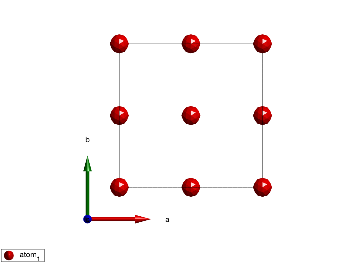
plot(model)
model.gencoupling
model.matom.r
Output
         0    0.5000    0.5000         0
         0    0.5000         0    0.5000
         0         0    0.5000    0.5000
model.table('bond',1)
Output
  24×10 table
    idx    subidx          dl                   dr             length     matom1     idx1     matom2     idx2        matrix
    ___    ______    ______________    ____________________    ______    ________    ____    ________    ____    ______________
    1       1         1     0     0     0.5    -0.5       0    3.182     'atom_1'    2       'atom_1'    1       ''    ''    ''
    1       2         0    -1     0     0.5    -0.5       0    3.182     'atom_1'    1       'atom_1'    2       ''    ''    ''
    1       3         0     0     0     0.5    -0.5       0    3.182     'atom_1'    4       'atom_1'    3       ''    ''    ''
    1       4         1    -1     0     0.5    -0.5       0    3.182     'atom_1'    3       'atom_1'    4       ''    ''    ''
    1       5         0     0     0    -0.5    -0.5       0    3.182     'atom_1'    2       'atom_1'    1       ''    ''    ''
    1       6        -1    -1     0    -0.5    -0.5       0    3.182     'atom_1'    1       'atom_1'    2       ''    ''    ''
    1       7        -1     0     0    -0.5    -0.5       0    3.182     'atom_1'    4       'atom_1'    3       ''    ''    ''
    1       8         0    -1     0    -0.5    -0.5       0    3.182     'atom_1'    3       'atom_1'    4       ''    ''    ''
    1       9         0     1     0       0     0.5    -0.5    3.182     'atom_1'    4       'atom_1'    1       ''    ''    ''
    1      10         0     0    -1       0     0.5    -0.5    3.182     'atom_1'    1       'atom_1'    4       ''    ''    ''
    1      11         0     0     0       0     0.5    -0.5    3.182     'atom_1'    3       'atom_1'    2       ''    ''    ''
    1      12         0     1    -1       0     0.5    -0.5    3.182     'atom_1'    2       'atom_1'    3       ''    ''    ''
    1      13         0     0     0       0    -0.5    -0.5    3.182     'atom_1'    4       'atom_1'    1       ''    ''    ''
    1      14         0    -1    -1       0    -0.5    -0.5    3.182     'atom_1'    1       'atom_1'    4       ''    ''    ''
    1      15         0    -1     0       0    -0.5    -0.5    3.182     'atom_1'    3       'atom_1'    2       ''    ''    ''
    1      16         0     0    -1       0    -0.5    -0.5    3.182     'atom_1'    2       'atom_1'    3       ''    ''    ''
    1      17         0     0     1    -0.5       0     0.5    3.182     'atom_1'    3       'atom_1'    1       ''    ''    ''
    1      18        -1     0     0    -0.5       0     0.5    3.182     'atom_1'    1       'atom_1'    3       ''    ''    ''
    1      19         0     0     0    -0.5       0     0.5    3.182     'atom_1'    2       'atom_1'    4       ''    ''    ''
    1      20        -1     0     1    -0.5       0     0.5    3.182     'atom_1'    4       'atom_1'    2       ''    ''    ''
    1      21         0     0     0    -0.5       0    -0.5    3.182     'atom_1'    3       'atom_1'    1       ''    ''    ''
    1      22        -1     0    -1    -0.5       0    -0.5    3.182     'atom_1'    1       'atom_1'    3       ''    ''    ''
    1      23         0     0    -1    -0.5       0    -0.5    3.182     'atom_1'    2       'atom_1'    4       ''    ''    ''
    1      24        -1     0     0    -0.5       0    -0.5    3.182     'atom_1'    4       'atom_1'    2       ''    ''    ''
According to the calculation there are 4 magnetic atoms in the crystallographic unit cell and 24 first neighbor bonds (6 per magnetic atom), here each bond is generated once. Details of the bond generation comes in the following section. Now we reduce the crystallographic unit cell to the primitive cell and compare the the result with the original model:
model.newcell('bvect',{[1/2 1/2 0] [1/2 0 1/2] [0 1/2 1/2]})
plot(model)
model.gencoupling
model.matom.r
Output
     0
     0
     0
model.table('bond',1)
Output
  6×10 table
    idx    subidx         dl               dr          length     matom1     idx1     matom2     idx2        matrix
    ___    ______    _____________    _____________    ______    ________    ____    ________    ____    ______________
    1      1         1     0    -1    1     0    -1    3.182     'atom_1'    1       'atom_1'    1       ''    ''    ''
    1      2         0    -1     1    0    -1     1    3.182     'atom_1'    1       'atom_1'    1       ''    ''    ''
    1      3         1    -1     0    1    -1     0    3.182     'atom_1'    1       'atom_1'    1       ''    ''    ''
    1      4         1     0     0    1     0     0    3.182     'atom_1'    1       'atom_1'    1       ''    ''    ''
    1      5         0     1     0    0     1     0    3.182     'atom_1'    1       'atom_1'    1       ''    ''    ''
    1      6         0     0     1    0     0     1    3.182     'atom_1'    1       'atom_1'    1       ''    ''    ''
The result is a primitive lattice with 1 magnetic atom and 6 bonds only. This is a very useful transformation for example if we want to calculate the spin wave dispersion of the FCC ferromagnet with Heisenberg exchange. In this case removing the symmetry operators does not change the Hamiltonian and the transformed model will contain only a single magnetic atom instead of 4 which will speed up the spin wave calculation. Another useful feature of the spinw.newcell method is that is generates the transformation matrix between reciprocal lattice vectors of the old and new unit cells, moreover this transformation matrix can be stored in the spinw object setting the keepq parameter to true. This means that after the transformation the spin wave dispersion can be still calculated using the original reciprocal lattice. This is useful when one wants to quickly compare a measurement indexed in the centered space group while the Hamiltonian is defined in the primitive cell.
Another useful symmetry transformation command is the spinw.nosym which reduces the symmetry to while keeping all the atoms. This can be used to generate starting lattices for distorted structures, since after the removal of symmetry all atomic positions are decoupled so they can be moved independently.
Atomic properties
Beside storing the position of the atoms and the spin quantum number, spinw store several other atomic properties attached to the symmetry inequivalent positions (see spinw.unit_cell). Some of these properties are unused at present, however we list here all of them for completeness. All atomic properties can be input into the spinw object using the spinw.addatom method.
The most important property is the magnetic form factor. spinw.addatom attempts to determine the magnetic form factor using the given label parameter. It searches the magion.dat file for matching labels and if found, the form factor coefficients are stored in the spinw.unit_cell.ff(1,:,i) matrix, where is the index of the atom. The magnetic form factor coefficients can be also given directly using the formfactn parameter of spinw.addatom by providing directly the coefficients , , , … in a row vector, where the magnetic form factor is calculated as
with .
There is also a color property assigned to each atom that can be input using the color parameter of the spinw.addatom method. Color can be given as an RGB triplet (integer values between 0-255) or as a string which is a valid color name in the color.dat file. The color will appear on the 3D structural plots (see swplot.plotatom).
To calculate density, spinw also stores the atomic number and atomic mass in the Z and A fields of spinw.unit_cell. For natural abundance of isotopes, use -1 as atomic mass. Information on isotope properties including neutron scattering cross section is stored in the isotope.dat file.